http://blog.outcome.io/pytorch-quick-start-classifying-an-image/

Data Loading and Processing Tutorial

Author: Sasank Chilamkurthy

튜토리얼 시작하기에 앞서 다음의 패키지를 다운받아야합니다

• scikit-image: For image io and transforms
• pandas: For easier csv parsing

다운방법

scikit-image:

https://anaconda.org/anaconda/scikit-image 참고

1. anaconda3 실행하여 가상환경 실행(activate '환경이름')

2. conda install -c anaconda scikit-image 입력하여 설치

pandas:

http://pandas.pydata.org/ 참고

1. anaconda3 실행하여 가상환경 실행(activate '환경이름')

2. conda install -c anaconda scikit-image 입력하여 설치

ARCNN을 공부하는 도중 이미지를 JPEG로 압축하기위해 오픈소스를 다운받았는데

scipy를 이용하는지라 이를 설치해야함

필자는 아나콘다로 가상환경을 만들고 파이참에서 그 가상환경을 기반으로

파이토치를 공부하기때문에 아나콘다로 만든 가상환경에 설치할 것이다

그 과정을 기록하였으며 대부분은 아래의 링크에서 참고하였습니다

http://pythonkim.tistory.com/78

1. numpy + mkl을 설치한다. https://www.lfd.uci.edu/~gohlke/pythonlibs/#numpy

에서 본인의 파이썬 버전과 윈도우 종류(32비트/64비트)에 따라 선택하여 whl파일 다운받는다

예) 파이썬 3.6, 윈도우 64비트라면 numpy-버전 + mkl-cp36-cp36m-win amd64.whl

2. Microsoft Visual C++ 2015 redistributable 설치

나는 2013과 2017이 깔려있었는데 2017에 필요한게 있어서인지 2015를 설치하려해도 이미 설치되어있다고 나와서 생략

3. scipy를 설치한다

https://www.lfd.uci.edu/~gohlke/pythonlibs/#scipy 에서 마찬가지로 버전에 맞는 걸 선택하여 다운받는다

예) 파이썬 3.6, 윈도우 64비트라면 scipy-버전-cp36-cp36m-win amd64.whl

4. 다운받은 두 whl파일을 C\사용자(Users)\사용자이름 폴더에 넣는다

아나콘다를 실행하여 pip install [whl 파일명] 으로 설치한다 .whl 까지 포함해서 입력

끝

http://ikaros0909.tistory.com/3

Learning PyTorch with Examples

파이토치 기본 컨셉을 소개하는 튜토리얼이다

파이토치가 제공하는 2가지 메인 특징:

n-차원 텐서는 넘파이와 비슷하지만 GPU들에서 돌릴 수 있다

신경망 형성과 학습에서 자동으로 differentiation

fully-connected ReLU 네트워크를 예시로 사용할 것이며

1개의 히든레이어가 있고, gradient descent 로 학습하여 임의의 데이터를 정답 결과와의 유클리안 거리를 최소화하는 방법으로 학습할 것

Tensors

파이토치에 앞서, 넘파이를 이용한 네트워크에 대한 내용

넘파이는 n차원 배열 오브젝트로, 이런 배열들을 계산하는 함수를 제공함 딥러닝이나 기울기 등에 대한 직접적인 것을 포함하진 않지만

넘파이 계산들을 이용하여 2개 레이어의 네트워크를 만들 수 있음

import numpy as np

N, D_in, H, D_out = 64, 1000, 100, 10

x = np.random.randn(N, D_in)
y = np.random.randn(N, D_out)

w1 = np.random.randn(D_in, H)
w2 = np.random.randn(H, D_out)

learning_rate = 1e-6

for t in range(500):
    #forward pass: predicted y 계산
    h = x.dot(w1)       #dot product? maybe
    h_relu = np.maximum(h, 0)       #normal ReLU
    y_pred = h_relu.dot(w2)

    #Compute and pritn loss
    loss = np.square(y_pred - y).sum()
    print(t, loss)

    #backprop to compute gradients of w1 and w2 with respect to loss
    grad_y_pred = 2.0 * (y_pred - y)
    grad_w2 = h_relu.T.dot(grad_y_pred)
    grad_h_relu = grad_y_pred.dot(w2.T)
    grad_h = grad_h_relu.copy()
    grad_h[h < 0] = 0
    grad_w1 = x.T.dot(grad_h)

    #update weights
    w1 -= learning_rate * grad_w1
    w2 -= learning_rate * grad_w2

PyTorch: Tensors

넘파이는 좋은 프레임웤이지만 GPU를 사용할 수 없음 최근 딥러닝 네트워크들은 GPU 사용시 50배 또는 그 이상 빨라지기도 하기때문에 넘파이 ㄴㄴ

파이토치 텐서는 넘파이랑 같음. n차원 배열이며 딥러닝에 대한 건 아니지만 배열에 대한 계산도 있고 쉽게 구현가능

하지만 넘파이와 달리 GPU를 이용하여 가속화할 수 있음 새로운 변수타입으로 cast하기만 하면 됨

다음은 텐서를 이용하여 2개 레이어 네트워크의 임의 데이터에 대한 학습을 하는 코드임

import torch

dtype = torch.float
device = torch.device("cpu")
# dtype = torch.device("cuda:0")        #GPU로 돌리려면 주석 해제

# N은 배치사이즈 D_in은 인풋 차원
# H는 히든 디멘션 D_out은 아웃풋 차원
N, D_in, H, D_out = 64, 1000, 100, 10

# Create random input and output data
x = torch.randn(N, D_in, device=device, dtype=dtype)
y = torch.randn(N, D_out, device=device, dtype=dtype)

# Randomly initialize weights
w1 = torch.randn(D_in, H, device=device, dtype=dtype)
w2 = torch.randn(H, D_out, device=device, dtype=dtype)

learning_rate = 1e-6
for t in range(500):
    # Forward pass: compute predicted y
    h = x.mm(w1)
    h_relu = h.clamp(min=0)
    y_pred = h_relu.mm(w2)

    # Compute and print loss
    loss = (y_pred - y).pow(2).sum().item()
    print(t, loss)

    # Backprop to compute gradients of w1 and w2 with respect to loss
    grad_y_pred = 2.0 * (y_pred - y)
    grad_w2 = h_relu.t().mm(grad_y_pred)
    grad_h_relu = grad_y_pred.mm(w2.t())
    grad_h = grad_h_relu.clone()
    grad_h[h < 0] = 0
    grad_w1 = x.t().mm(grad_h)

    # Update weights using gradient descent
    w1 -= learning_rate * grad_w1
    w2 -= learning_rate * grad_w2

Autograd

위 코드에서 수동적으로 네트워크 학습을 진행시켰는데 좀만 복잡해져도 힘들어짐. 

다행히도 automatic differentiation 을 이용해서 신경망 backward pass를 자동으로 계산할 수 있음 파이토치에서는 autograd 패키지를 이용

네트워크 정방향 진행하면 computational 그래프가 정의됨. 그래프의 노드는 텐서들이며 엣지는 아웃풋 텐서를 만드는 계산식. Backpropagation

시 기울기 계산하기가 쉬워짐

복잡한 소리처럼 들리지만, 사용하기엔 간단함

x 텐서 변수가 x.requires_grad=True라면 x.grad는 이 x의 기울기값을 담는 텐서임

아래 코드는 이전 코드에서 필요한부분만 autograd 패키지를 이용하는쪽으로 수정한 코드임:

import torch

dtype = torch.float
device = torch.device("cpu")
# dtype = torch.device("cuda:0")        #GPU로 돌리려면 주석 해제

# N은 배치사이즈 D_in은 인풋 차원
# H는 히든 디멘션 D_out은 아웃풋 차원
N, D_in, H, D_out = 64, 1000, 100, 10

# Create random input and output data
x = torch.randn(N, D_in, device=device, dtype=dtype)
y = torch.randn(N, D_out, device=device, dtype=dtype)

# Randomly initialize weights
w1 = torch.randn(D_in, H, device=device, dtype=dtype, requires_grad=True)
w2 = torch.randn(H, D_out, device=device, dtype=dtype, requires_grad=True)

learning_rate = 1e-6
for t in range(500):
    # # Forward pass: compute predicted y
    # h = x.mm(w1)
    # h_relu = h.clamp(min=0)
    # y_pred = h_relu.mm(w2)
    y_pred = x.mm(w1).clamp(min=0).mm(w2)

    # Compute and print loss
    #loss = (y_pred - y).pow(2).sum().item()
    loss = (y_pred - y).pow(2).sum()
    print(t, loss.item())

    # # Backprop to compute gradients of w1 and w2 with respect to loss
    # grad_y_pred = 2.0 * (y_pred - y)
    # grad_w2 = h_relu.t().mm(grad_y_pred)
    # grad_h_relu = grad_y_pred.mm(w2.t())
    # grad_h = grad_h_relu.clone()
    # grad_h[h < 0] = 0
    # grad_w1 = x.t().mm(grad_h)
    loss.backward()

    with torch.no_grad():
        w1 -= learning_rate * w1.grad
        w2 -= learning_rate * w2.grad

        #수동으로 기울기를 0으로 다시 해줌
        w1.grad.zero_()
        w2.grad.zero_()

    # # Update weights using gradient descent
    # w1 -= learning_rate * grad_w1
    # w2 -= learning_rate * grad_w2

PyTorch: Defining new autograd functions

각각의 오토그래드 기본 계산은 사실 텐서를 계산하는 두개의 함수이다. 

forward 함수는 인풋 텐서로부터 아웃풋 텐서를 계산한다.

backward 함수는 아웃풋 텐서의 기울기를 받아 인풋 텐서의 기울기를 계산한다.

torch.autograd.Function 의 서브클래스를 정의하고 forward와 backward 함수를 시행하여 우리는 우리만의 autograd 연산을 만들 수 있다. 

그리고 인스턴스를 생성하고 함수처럼 생성하여 우리의 새로운 연산을 이용해서 인풋데이터를 포함하는 텐서를 넘긴다

아래 예제에서 우리의 커스텀 오토그래드 함수를 정의하여 ReLU nonlinearity를 수행하고 2개 레이어 네트워크를 실행한다

# -*- coding: utf-8 -*-

import torch

class MyReLU(torch.autograd.Function):
    """
    서브클래스를 생성하여 고유의 오토그래드 함수를 만듦
    """
    @staticmethod
    def forward(ctx, input):
        """
        forward 패스에서 인풋이 담긴 텐서를 받아 아웃풋이 담긴 텐서를 반환한다. ctx는 context object이며 backward 계산을
        위한 정보를 숨기는데 사용한다. ctx.save_for_backward를 이용해서 backward pass에 사용하기위해 임의의 오브젝트를 캐시
        """
        ctx.save_for_backward(input)
        return input.clamp(min=0)

    @staticmethod
    def backward(ctx, grad_output):
        """
        backward 패스에서 아웃풋쪽 loss의 gradient를 담는 텐서를 받아 input쪽 기울기를 계산해야함
        """
        input, = ctx.saved_tensors
        grad_input = grad_output.clone()
        grad_input[input < 0] = 0
        return grad_input

dtype = torch.float
device = torch.device("cpu")

# N is batch size; D_in is input dimension;
# H is hidden dimension; D_out is output dimension.
N, D_in, H, D_out = 64, 1000, 100, 10

# Create random Tensors to hold input and outputs.
x = torch.randn(N, D_in, device=device, dtype=dtype)
y = torch.randn(N, D_out, device=device, dtype=dtype)

# Create random Tensors for weights.
w1 = torch.randn(D_in, H, device=device, dtype=dtype, requires_grad=True)
w2 = torch.randn(H, D_out, device=device, dtype=dtype, requires_grad=True)

learning_rate = 1e-6
for t in range(500):
    # 우리가 만든 함수를 사용하기 위해 .apply를 사용함 우리는 이걸 relu라 부름
    relu = MyReLU.apply

    # forward 패스: y를 예상하여 계산함; 우리가 계산함
    # ReLu 는 우리 고유 함수를 이용한것
    y_pred = relu(x.mm(w1)).mm(w2)

    # loss 계산하고 출력
    loss = (y_pred - y).pow(2).sum()
    print(t, loss.item())

    loss.backward()

    # gradient descent를 이용하여 weights 갱신
    with torch.no_grad():
        w1 -= learning_rate * w1.grad
        w2 -= learning_rate * w2.grad

        w1.grad.zero_()
        w2.grad.zero_()

TensorFlow: Static Graphs

파이토치는 텐서플로우와 매우 비슷함. 둘다 computational 그래프를 만들고, automatic differentiation 을 사용하여 기울기 계산함

가장 큰 차이점은 그래프가 텐서플로우는 static이고 파이토치는 dynamic

텐서플로우에서 그래프를 생성하고 이걸 계속 같은걸 쓰고 또 씀. 인풋데이터만 다르게 줘서말이지.

파이토치는 각각의 forward pass가 각각의 그래프를 생성함

static 그래프는 개발자가 optimize하는 측면에서 더 나이스함. 예를들어 프레임워크는 일부 그래프 연산을 효율을 위해 융합(fuse)시키거나

여러 GPU나 머신들에게 분배하는 전력을 쓸 수 있음. 만약 같은 그래프를 계속 반복해서 다시 사용한다면 이건 비용적으로 선행 optimization이

분할상환될 수 있음(이 부분 한정 직역)

static과 dynamic 그래프가 다른 것 중 하나는 control flow이다. 일부 모델들에서는 각각의 데이터 포인트에 따라 다른 계산을 하길 바랄 수도 있다.

예를들어 반복네트워크(Recurrent Network - RNN)에서 각각의 데이터포인트에서 시간 단계에 따라 다르기 때문에 펼쳐질 수 있다

이 펼치는건 loop 반복으로 시행될 수 있다. static 그래프에서 반복되는 부분은 그래프의 일부여야 한다. 이러한 이유에서 텐서플로우에서는 tf.scan 같은 연산을 제공하여 그래프에 내장된 루프를 시행한다.

dynamic 그래프에선 더 간단하다. 각각의 예시에 대해 그래프를 생성하기때문에 일반적인 긴요한 플로우 컨트롤을 사용하여 각각의 인풋에 맞게

연산을 할 수 있다.

이전의 autograd 예시와 비교하기 위해 여기서는 텐서플로우를 이용하여 2개 레이어 네트워크를 학습하였다

# -*- coding: utf-8 -*-
import tensorflow as tf
import numpy as np

# First we set up the computational graph:

# N is batch size; D_in is input dimension;
# H is hidden dimension; D_out is output dimension.
N, D_in, H, D_out = 64, 1000, 100, 10

# Create placeholders for the input and target data; these will be filled
# with real data when we execute the graph.
x = tf.placeholder(tf.float32, shape=(None, D_in))
y = tf.placeholder(tf.float32, shape=(None, D_out))

# Create Variables for the weights and initialize them with random data.
# A TensorFlow Variable persists its value across executions of the graph.
w1 = tf.Variable(tf.random_normal((D_in, H)))
w2 = tf.Variable(tf.random_normal((H, D_out)))

# Forward pass: Compute the predicted y using operations on TensorFlow Tensors.
# Note that this code does not actually perform any numeric operations; it
# merely sets up the computational graph that we will later execute.
h = tf.matmul(x, w1)
h_relu = tf.maximum(h, tf.zeros(1))
y_pred = tf.matmul(h_relu, w2)

# Compute loss using operations on TensorFlow Tensors
loss = tf.reduce_sum((y - y_pred) ** 2.0)

# Compute gradient of the loss with respect to w1 and w2.
grad_w1, grad_w2 = tf.gradients(loss, [w1, w2])

# Update the weights using gradient descent. To actually update the weights
# we need to evaluate new_w1 and new_w2 when executing the graph. Note that
# in TensorFlow the the act of updating the value of the weights is part of
# the computational graph; in PyTorch this happens outside the computational
# graph.
learning_rate = 1e-6
new_w1 = w1.assign(w1 - learning_rate * grad_w1)
new_w2 = w2.assign(w2 - learning_rate * grad_w2)

# Now we have built our computational graph, so we enter a TensorFlow session to
# actually execute the graph.
with tf.Session() as sess:
    # Run the graph once to initialize the Variables w1 and w2.
    sess.run(tf.global_variables_initializer())

    # Create numpy arrays holding the actual data for the inputs x and targets
    # y
    x_value = np.random.randn(N, D_in)
    y_value = np.random.randn(N, D_out)
    for _ in range(500):
        # Execute the graph many times. Each time it executes we want to bind
        # x_value to x and y_value to y, specified with the feed_dict argument.
        # Each time we execute the graph we want to compute the values for loss,
        # new_w1, and new_w2; the values of these Tensors are returned as numpy
        # arrays.
        loss_value, _, _ = sess.run([loss, new_w1, new_w2],
                                    feed_dict={x: x_value, y: y_value})
        print(loss_value)

nn module

Computational graph나 autograd는 복잡한 연산을 정의하고 자동으로 기울기를 구하기위해 매우 파워풀한 패러다임. 하지만

거대한 신경망에서 autograd는 약간 low-level일 수 있음

텐서플로우에서 Keras, TensorFlow-Slim, 등과 같은 패키지는 좀더 높은 레벨(higher-level)의 관념을 제공하여 신경망 만들때 더 유용함

파이토치에서는 nn 패키지가 같은 목적으로 이용됨. Modules의 집합을 정의하며 이건 신경망의 레이어에 해당함. 하나의 모듈은 인풋 텐서를 받아

아웃풋 텐서를 계산하지만 학습할 파라미터를 포함한 텐서같은 것을 내부 state로 가지고있기도 함

nn 패키지는 또한 신경망 학습 시 일반적으로 많이 사용하는 loss 함수들도 정의함

아래 예시는 2개 레이어 네트워크를 nn패키지를 이용하여 구성한것

import torch

N, D_in, H, D_out = 64, 1000, 100, 10

x = torch.randn(N, D_in)
y = torch.randn(N, D_out)

# nn 패키지를 이용하여 레이어를 나열하여 모델을 만듬. nn.Sequential 은 다른 모듈을 포함하는 모듈이고
# 이를 적용하여 output을 얻어냄. 각각의 선형 모듈은 인풋으로부터 선형 함수를 이용하여 아웃풋을 계산
# 그리고 weight과 bias를 홀드
model = torch.nn.Sequential(
    torch.nn.Linear(D_in, H),
    torch.nn.ReLU(),
    torch.nn.Linear(H, D_out),
)

# nn 패키지는 유명한 몇개의 loss 함수도 갖고있음
loss_fn = torch.nn.MSELoss(size_average=False)

learning_rate=1e-4
for t in range(500):
    # x를 모델로 통과시켜서 y를 예측하여 게산함. 모듈 오브젝트는 __call__ 연산을 오버라이드하여 함수처럼 호출하게함
    # 인풋과 아웃풋은 텐서임
    y_pred = model(x)

    # 로스 계산과 출력. 계산된 y와 실제 y를 포함하는 텐서들을 넘기면 계산해줌
    loss = loss_fn(y_pred, y)
    print(t, loss.item())

    # 기울기 0으로 만들기 backward pass 하기 전에
    model.zero_grad()

    # backward pass: 모델의 학습가능한 모든 파라미터에 대해 기울기 계산하고, 각각 모듈(레이어)의 파라미터는 텐서에
    #저장되어있음 requires_grad=True 속성을 호출하면 모든 기울기를 계산할것임
    loss.backward()

    # gradient descent 이용하여 weight들 업데이트함
    with torch.no_grad():
        for param in model.parameters():
            param -= learning_rate * param.grad

PyTorch: optim

파이토치의 optim 패키지는 optimization 알고리즘의 아이디어를 추상화하고 널리 사용되는 알고리즘을 제공한다.

아래 코드는 nn패키지로 모델을 정의하고 optim패키지가 제공하는 Adam 알고리즘으로 optimize 하는것이다

import torch

# N is batch size; D_in is input dimension;
# H is hidden dimension; D_out is output dimension.
N, D_in, H, D_out = 64, 1000, 100, 10

# Create random Tensors to hold inputs and outputs
x = torch.randn(N, D_in)
y = torch.randn(N, D_out)

# Use the nn package to define our model and loss function.
model = torch.nn.Sequential(
    torch.nn.Linear(D_in, H),
    torch.nn.ReLU(),
    torch.nn.Linear(H, D_out),
)
loss_fn = torch.nn.MSELoss(size_average=False)

# optim 패키지의 Adam 알고리즘을 이용하여 optimize함. 다른 알고리즘도 많음
# Adam 알고리즘의 첫번째 인자는 어떤 텐서를 아담이 업데이트해야하는지 알려줌

learning_rate = 1e-4
optimizer = torch.optim.Adam(model.parameters(), lr=learning_rate)
for t in range(500):
    # Forward pass: compute predicted y by passing x to the model.
    y_pred = model(x)

    # Compute and print loss.
    loss = loss_fn(y_pred, y)
    print(t, loss.item())

    # backward pass 하기 전에, 모든 기울기를 0으로 만들어야하는데 왜냐하면 .backward()가 호출이되면 기본값으로
    # 기울기값들은 버퍼에 축적되기때문
    optimizer.zero_grad()

    # backward pass: 모델 파라미터에 따른 loss 기울기 계산
    loss.backward()

    #step 함수는 파라미터를 갱신함
    optimizer.step()

PyTorch: Custom nn Modules

기존에 존재하는 모듈 외에 좀더 복잡한 모델을 원할 경우가 있을텐데 이때는 nn.Module이라는 서브클래스로 고유한 모듈을 만들 수 있다. 

import torch

class TwoLayerNet(torch.nn.Module):
    def __init__(self, D_in, H, D_out):
        """
        2개의 nn.Linear 모듈(레이어)를 초기화하고 멤버 변수 할당화
        :param D_in:
        :param H:
        :param D_out:
        """
        super(TwoLayerNet, self).__init__()
        self.linear1 = torch.nn.Linear(D_in, H)
        self.linear2 = torch.nn.Linear(H, D_out)

    def forward(self, x):
        """
        인풋 텐서를 받아서 아웃풋 텐서를 반환해야함 생성자에 정의된 모듈이나 텐서의 임의 연산을 사용할 수 있음
        :param x:
        :return:
        """
        h_relu = self.linear1(x).clamp(min=0)
        y_pred = self.linear2(h_relu)
        return y_pred

# N is batch size; D_in is input dimension;
# H is hidden dimension; D_out is output dimension.
N, D_in, H, D_out = 64, 1000, 100, 10

# Create random Tensors to hold inputs and outputs
x = torch.randn(N, D_in)
y = torch.randn(N, D_out)

# Construct our model by instantiating the class defined above
model = TwoLayerNet(D_in, H, D_out)

# Loss 함수와 Opimizer를 정의함. model.parameters()를 호출하여 SGD를 사용하면 모델의 레이어들의 학습해야할 파라미터가 넘겨짐
criterion = torch.nn.MSELoss(size_average=False)
optimizer = torch.optim.SGD(model.parameters(), lr=1e-4)
for t in range(500):
    # forward pass: y 예상값을 계산함 x를 모델에 통과시켜서
    y_pred = model(x)

    loss = criterion(y_pred, y)
    print(t, loss.item())

    # 기울기 0, backward pass, weights 갱신
    optimizer.zero_grad()
    loss.backward()
    optimizer.step()

PyTorch: Control Flow + Weight Sharing

dynamic 그래프와 weight 공유의 예로 상당히 이상한 모델을 돌려봅시다. fully-connected ReLU 네트워크이며 각각의 패스에서 1부터 4 사이의 숫자를 고르고 그 숫자만큼의(?) 히든레이어를 사용하며 같인 weights를 여러번 사용하여 가장 안쪽에있는 히든레이어를 계산함

루프를 돌리기 위해 일반적인 파이썬 플로우 컨트롤을 사용하며 forward pass 선언 시 같은 모듈을 여러번 사용함으로써 weights를 공유함

모듈 서브클래스를 이용하면 쉽게 시행할 수 있음

import random
import torch

class DynamicNet(torch.nn.Module):
    def __init__(self, D_in, H, D_out):
        """
        생성자에서 3개 nn.Linear 인스턴스를 생성하여 forward pass에서 사용할것
        :param D_in:
        :param H:
        :param D_out:
        """
        super(DynamicNet, self).__init__()
        self.input_linear = torch.nn.Linear(D_in, H)
        self.middle_linear = torch.nn.Linear(H, H)
        self.output_linear = torch.nn.Linear(H, D_out)

    def forward(self, x):
        """
        forward 패스에서 0~3까지 골라 그 숫자만큼 중간 레이어를 반복하여 히든레이어를 계산함
        각각의 pass가 그래프를 생성하므로 파이썬의 반복문이나 조건문 등의 일반적인 컨트롤 플로우 연산자를
        사용하여 모델의 forward 패스를 구현 가능함

        또한 computational graph를 생성하는데 있어 같은 모듈을 여러번 사용해도 안전함 LuaTorch 대비 가장 발전한 부분
        :param x:
        :return:
        """
        h_relu = self.input_linear(x).clamp(min=0)
        for _ in range(random.randint(0, 3)):
            h_relu = self.middle_linear(h_relu).clamp(min=0)
        y_pred = self.output_linear(h_relu)
        return y_pred

# N is batch size; D_in is input dimension;
# H is hidden dimension; D_out is output dimension.
N, D_in, H, D_out = 64, 1000, 100, 10

# Create random Tensors to hold inputs and outputs
x = torch.randn(N, D_in)
y = torch.randn(N, D_out)

# Construct our model by instantiating the class defined above
model = DynamicNet(D_in, H, D_out)

# 이 이상한 모델을 vanilla stochastic gradient descent로 하기엔 너무 터프하니 momentum 이용
# SGD - stochastic gradient descent
# 최적화 관련 용어 : http://ikaros0909.tistory.com/3
criterion = torch.nn.MSELoss(size_average=False)
optimizer = torch.optim.SGD(model.parameters(), lr=1e-4, momentum=0.9)
for t in range(500):
    # Forward pass: Compute predicted y by passing x to the model
    y_pred = model(x)

    # Compute and print loss
    loss = criterion(y_pred, y)
    print(t, loss.item())

    # Zero gradients, perform a backward pass, and update the weights.
    optimizer.zero_grad()
    loss.backward()
    optimizer.step()

Authors: Sung Kim and Jenny Kang

2개이상의 GPU를 DataParallel을 이용하여 사용하는 법

우선 GPU에 모델을 전달하는 방법은 매우 쉬움

device = torch.device("cuda:0")
model.to(device)

그리고, 모든 텐서를 GPU로 복사

mytensor = my_tensor.to(device)

my_tensor.to(device)는 mytensor를 새로 쓰는게 아니라 값을 복사해서 넘김

따라서 이걸 mytensor라는 새로운 변수에 할당해야하는듯

모델의 학습과정을 여러대의 GPU로 이용하는것은 자연스러워 보이지만 파이토치는 1개만 사용하는것을 디폴트로함

따라서 DataParallel 을 이용하여 여러대의 GPU 로 돌릴 수 있음

model = nn.DataParallel(model)

이게 이번 강의의 핵심

Imports and parameters

모듈 임포트 및 변수 정의

import torch
import torch.nn as nn
from torch.utils.data import Dataset, DataLoader

input_size = 5
output_size = 2

batch_size = 30
data_size = 100

device = torch.device("cuda:0" if torch.cuda.is_available() else "cpu")

Dummy DataSet

임의의 데이터셋을 만듬. getitem만 추가해주면 됨

class RandomDataset(Dataset):
    def __init__(self, size, length):
        self.len = length
        self.data = torch.randn(length, size)
        
    def __getitem(self, index):
        return self.data[index]
    
    del __len__(self):
        return self.len

rand_loader = DataLoader(dataset=RandomDataset(input_size, 100), batch_size=batch_size, shuffle=True)

Simple Model

이번 강의에 쓸 모델은 단순히 인풋을 넣으면 선형 연산을 하고 아웃풋을 줌 하지만 CNN, RNN, 등 어떤 모델에서도 DataParallel을 쓸 수 있음

print 메소드는 인풋 아웃풋 텐서 사이즈를 알아보기 위해 넣었음. batch rank 0 일때 뭐가 출력되는지 주의해서 볼것

모델 정의:

class Model(nn.Module):
    def __init__(self, input_size, output_size):
        super(Model, self).__init__()
        self.fc = nn.Linear(input_size, output_size)
        
    def forward(self, input):
        output = self.fc(input)
        print("\tIn Model: input size", input.size(), "output size", output.size())
        
        return output

Create Model and DataParallel

model = Model(input_size, output_size)
if torch.cuda.device_count() > 1:
    print("Let's use", torch.cuda.device_count(), "GPUs!")
    model = nn.DataParallel(model)

model.to(device)

Run the Model

인풋,아웃풋 텐서들의 사이즈를 볼 수 있음

GPU가 하나라 하지 않았음

우선, 제 경우 numpy, matplotlib 설치시도하고, cython을 필요로하다는 빨간색 메세지가 떠서

이후에 cython 설치 후 다시 numpy와 matplotlib를 설치(이때, 모든 것이 이미 설치되어있다고 나옴 cython이 필수는 아닌듯)

아나콘다 실행하여 가상환경 활성화함 (activate envname)

https://anaconda.org/anaconda/cython

참조하여 가상환경에 cython 설치

이후 

pip install numpy

pip install matplotlib 명령어로 설치 ( 둘다 전부 이미 설치되어있다고 나옴)

Training a classifier

What about data

이미지,텍스트,av(audio and video) 데이터에 대해 다룰 때에는, 표준 파이썬 패키지를 사용하여 해당 데이터를 numpy 배열로 불러올수있습니다

그리고 이 배열을 torch.Tensor로 변환할 수 있습니다

이미지들은 Pillow, OpenCV 같은 패키지가 유용합니다

오디오는 scipy, librosa 같은 패키지가 유용합니다

텍스트는 raw레벨의 파이썬이나 Cython으로 불러오거나 NLTK, SpaCy 등이 유용합니다

Imagenet, CIFAR10, MNIST 와 같은 일반적인 데이터셋을 불러오기 위해서 torchvision이라는 패키지가 있습니다

이미지나 viz 등을 위한 데이터 변환기(transformer)로 torchvision.datasets와 torch.utils.data.DataLoader가 있습니다

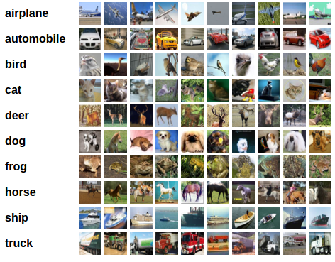
이 튜토리얼에서는 CIFAR10데이터셋을 이용할것입니다. 이 데이터셋의 클래스에는 '비행기', '자동차', '새', '고양이', '사슴', 

개', '개구리', '말', '배', '트럭'가 있고 사이즈는 3x32x32입니다 (32x32 픽셀의 3채널 이미지)

Training an image classifier

순서:

1. CIFAR10 학습 및 테스트 데이터셋을 torchvision을 이용하여 불러오고 정규화(normalizing) 합니다

2. CNN을 정의합니다

3. 로스 함수를 정의합니다

4. 학습 셋으로 네트워크를 학습합니다

5. 테스트 셋으로 네트워크를 테스흡니다

1. Loading and normalizing CIFAR10

torchvision을 이용하여 매우 쉽게 CIFAR10을 불러올 수 있습니다

import torch
import torchvision
import torchvision.transforms as transforms

토치비전 데이터셋의 아웃풋은 PILImage이며 범위는 [0,1] 입니다. 이걸 [-1, 1] 범위의 텐서로 정규화합니다

우선 아래의 코드로 CIFAR10을 다운받아 로드합니다

#데이터 가져오기

trainset = torchvision.datasets.CIFAR10(root = './data', train=True, download=True, transform = transform)
trainloader = torch.utils.data.DataLoader(trainset, batch_size=4, shuffle=True, num_workers=2)
testset = torchvision.datasets.CIFAR10(root = './data', train=False, download=True, transform=transform)
testloader = torch.utils.data.DataLoader(testset, batch_size=4, shuffle=False, num_workers=2)

classes = ('plane', 'car', 'bird', 'cat', 'deer', 'dog', 'frog', 'horse', 'ship', 'truck')

실행(ctrl + shift + F10)하고 조금 기다리면 데이터셋을 받고 압축을 풉니다 경로는 프로젝트 설치경로(보통 users/이름/PycharmProjects/프로젝트이름/data

아래 코드로 학습 셋 중 일부를 로드하려고 했는데 이 과정에서 matplotlib와 numpy 가 없어 설치하였음 아래 글 참조

http://busterworld.tistory.com/61?category=663469

import matplotlib.pyplot as plt
import numpy as np

# functions to show an image


def imshow(img):
    img = img / 2 + 0.5     # unnormalize
    npimg = img.numpy()
    plt.imshow(np.transpose(npimg, (1, 2, 0)))


# get some random training images
dataiter = iter(trainloader)
images, labels = dataiter.next()

# show images
imshow(torchvision.utils.make_grid(images))
# print labels
print(' '.join('%5s' % classes[labels[j]] for j in range(4)))

*이 코드 입력시 쓰레드 관련 에러가 뜹니다. 그 이유는, 위에 데이터 가져오는 코드에서 num_workers=2 로 하여 2개 쓰레드를 이용해서

데이터를 로드했는데 로드가 끝나기 전에 trainloader를 이용해서 작업을 시도했기때문인것으로 생각되고

num_workers=0으로 고치거나, 아래 이미지 불러오는 코드에 조건문 if __name__ == '__main__': 으로 제어를 하면

해결됩니다(단, 조건문을 넣는거보다 0으로 고치는게 속도가 더 빠르네요)

*또한, 불러온 4개 이미지를 보여주기위해서 맨아래에 plt.show()를 추가했습니다 원래 코드만 작성하면 이미지를 보여주진않네요

2. Define a Convolution Neural Network

이전의 NN에서 1채널 대신 3채널 이미지를 사용하는것으로 변경

3. Define a Loss function and optimizer

Classification Cross-Entropy loss와 momentum을 포함한 SGD를 사용

4. Train the network

학습시키기

for epoch in range(2):  # loop over the dataset multiple times

    running_loss = 0.0
    for i, data in enumerate(trainloader, 0):
        # get the inputs
        inputs, labels = data

        # zero the parameter gradients
        optimizer.zero_grad()

        # forward + backward + optimize
        outputs = net(inputs)
        loss = criterion(outputs, labels)
        loss.backward()
        optimizer.step()

        # print statistics
        running_loss += loss.item()
        if i % 2000 == 1999:    # print every 2000 mini-batches
            print('[%d, %5d] loss: %.3f' %
                  (epoch + 1, i + 1, running_loss / 2000))
            running_loss = 0.0

print('Finished Training')

[1,  2000] loss: 2.199
[1,  4000] loss: 1.856
[1,  6000] loss: 1.688
[1,  8000] loss: 1.606
[1, 10000] loss: 1.534
[1, 12000] loss: 1.488
[2,  2000] loss: 1.420
[2,  4000] loss: 1.384
[2,  6000] loss: 1.336
[2,  8000] loss: 1.351
[2, 10000] loss: 1.309
[2, 12000] loss: 1.277
Finished Training

5. Test the network on the test data

2개 패스로 학습을 시켰으니 확인을 해봐야겠쥬?

클래스를 에측해보고, 맞으면 그 샘플을 리스트에 추가할겁니다

dataiter = iter(testloader)
images, labels = dataiter.next()

# print images
imshow(torchvision.utils.make_grid(images))
print('GroundTruth: ', ' '.join('%5s' % classes[labels[j]] for j in range(4)))

이제 신경망이 이 이미지에 대해 어떻게 판단하는지 봅니다

outputs = net(images)

outputs는 10개 클래스에 대한 에너지들인데 에너지가 높을수록 네트워크는 해당 클래스라고 생각한다는것 따라서 가장 높은것의 인덱스를 가져옴

_, predicted = torch.max(outputs, 1)

print('Predicted: ', ' '.join('%5s' % classes[predicted[j]] for j in range(4)))

또한 전체 데이터셋(테스트셋)에 대한 정확도를 알아보는 코드:

correct = 0
total = 0
with torch.no_grad():
    for data in testloader:
        images, labels = data
        outputs = net(images)
        _, predicted = torch.max(outputs.data, 1)
        total = labels.size(0)
        correct += (predicted == labels).sum().item()

print('Accuracy of the network on the 10000 test images: %d %%' % (100 * correct / total))

53%의 정확도를 보이는데, 랜덤하게 찍는 확률인 10%보단 훨씬 좋음. 네트워크가 뭔가를 배우고있긴함

클래스별 정확도를 araboza:

class_correct = list(0. for i in range(10))
class_total = list(0. for i in range(10))

with torch.no_grad():
    for data in testloader:
        images, labels = data
        outputs = net(images)
        _, predicted = torch.max(outputs, 1)
        c = (predicted == labels).squeeze()
        for i in range(4):
            label = labels[i]
            class_correct[label] += c[i].item()
            class_total[label] += 1

for i in range(10):
    print('Accuracy of %5s : %2d %%' % (classes[i], 100 * class_correct[i] / class_total[i]))

전체 정확도는 54퍼, 클래스별은 위와 같이 나옴 

이제 GPU에서 돌려보자:

Training on GPU

텐서를 GPU로 전달하는 거처럼 신경망도 GPU로 전달 가능함

우선 CUDA 가능한지 보고 기기를 부여해야함

device = torch.device("cuda:0" if torch.cuda.is_available() else "cpu")

# Assume that we are on a CUDA machine, then this should print a CUDA device:

print(device)

Out:

cuda:0

그리고 메소드들은 모든 모듈에 재귀적으로 동작하여야하며 파라미터와 버퍼를 CUDA 텐서로 바꾸어야함

이라고하면서

net.to(device)

라던지, 인풋과 타겟을 모든 단계에서 GPU로 보내야한다며

inputs, labels = inputs.to(device), labels.to(device)

이렇게 해놓고 설명 끝인데, 이 두 구문을 어디다 넣을것인가??

그 힌트는 https://github.com/MorvanZhou/PyTorch-Tutorial/blob/master/tutorial-contents/502_GPU.py

에 있는줄..알았는데 조금 다르다 직접 고민해보고 업데이트하자

우선 지금까지 cpu용으로 해온것 정리:

데이터셋 가져오기 - CIFAR10으로 트레이닝셋, 테스트셋만들기

신경망 정의

로스, 옵티마이저 정의 - CrossEntropyLoss, SGD 모멘텀 0.9

에포크 2 학습 꼬우

테스트

정확도 평가

이 과정을 정리한 소스코드는 다음과 같다:

import torch
import torchvision
import torchvision.transforms as transforms
import torch.nn as nn
import torch.nn.functional as F
import matplotlib.pyplot as plt
import numpy as np
import torch.optim as optim

transform = transforms.Compose(
    [transforms.ToTensor(),
     transforms.Normalize((0.5, 0.5, 0.5), (0.5, 0.5, 0.5))])

#데이터 가져오기

trainset = torchvision.datasets.CIFAR10(root = './data', train=True, download=True, transform = transform)
trainloader = torch.utils.data.DataLoader(trainset, batch_size=4, shuffle=True, num_workers=0)
testset = torchvision.datasets.CIFAR10(root = './data', train=False, download=True, transform=transform)
testloader = torch.utils.data.DataLoader(testset, batch_size=4, shuffle=False, num_workers=0)

classes = ('plane', 'car', 'bird', 'cat', 'deer', 'dog', 'frog', 'horse', 'ship', 'truck')

def imshow(img):
    img = img / 2 + 0.5
    npimg = img.numpy()
    plt.imshow(np.transpose(npimg, (1, 2, 0)))

class Net(nn.Module):
    def __init__(self):
        super(Net, self).__init__()
        self.conv1 = nn.Conv2d(3, 6, 5)
        self.pool = nn.MaxPool2d(2, 2)
        self.conv2 = nn.Conv2d(6, 16, 5)
        self.fc1 = nn.Linear(16 * 5 * 5, 120)
        self.fc2 = nn.Linear(120, 84)
        self.fc3 = nn.Linear(84, 10)

    def forward(self, x):
        x = self.pool(F.relu(self.conv1(x)))
        x = self.pool(F.relu(self.conv2(x)))
        x = x.view(-1, 16 * 5 * 5)
        x = F.relu(self.fc1(x))
        x = F.relu(self.fc2(x))
        x = self.fc3(x)
        return x


net = Net()

#loss function, optimizer
criterion = nn.CrossEntropyLoss()
optimizer = optim.SGD(net.parameters(), lr=0.001, momentum=0.9)

#Training
for epoch in range(2):

    running_loss = 0.0
    for i, data in enumerate(trainloader, 0):
        #인풋 가져오기
        inputs, labels = data

        #gradient 0으로
        optimizer.zero_grad()

        #forward + backward + optimize
        outputs = net(inputs)
        loss = criterion(outputs, labels)
        loss.backward()
        optimizer.step()

        #통계 출력
        running_loss += loss.item()
        if i % 2000 == 1000: #2000 미니배치마다 출력
            print('[%d, %5d] loss: %.3f' % (epoch + 1, i + 1, running_loss / 2000))
            running_loss = 0.0
print('Finished Training')

#테스트 해봅시다
dataiter = iter(testloader)
images, labels = dataiter.next()

# print images
imshow(torchvision.utils.make_grid(images))
print('GroundTruth: ', ' '.join('%5s' % classes[labels[j]] for j in range(4)))

#테스트 돌림
outputs = net(images)

_, predicted = torch.max(outputs, 1)

print('Predicted: ', ' '.join('%5s' % classes[predicted[j]] for j in range(4)))

#정확도 평가
correct = 0
total = 0
class_correct = list(0. for i in range(10))
class_total = list(0. for i in range(10))

with torch.no_grad():
    for data in testloader:
        images, labels = data
        outputs = net(images)
        _, predicted = torch.max(outputs.data, 1)
        c = (predicted == labels).squeeze()
        for i in range(4):
            label = labels[i]
            class_correct[label] += c[i].item()
            class_total[label] += 1
        total += labels.size(0)
        correct += (predicted == labels).sum().item()

print('Accuracy of the network on the 10000 test images: %d %%' % (100 * correct / total))

for i in range(10):
    print('Accuracy of %5s : %2d %%' % (classes[i], 100 * class_correct[i] / class_total[i]))


plt.show()

GPU로 돌리는것을 일단 짜긴 짰는데

아직 잘 다루지 않아서인지, 네트워크가 작아서인지 CPU보다 (당연히) 오래걸리는것 같다

신경망 net을 GPU로 보내고

학습이나 테스트 돌릴때 즉, 신경망을 사용할때 파라미터들을 GPU로 보내어 돌렸다

import torch
import torchvision
import torchvision.transforms as transforms
import torch.nn as nn
import torch.nn.functional as F
import matplotlib.pyplot as plt
import numpy as np
import torch.optim as optim

transform = transforms.Compose(
    [transforms.ToTensor(),
     transforms.Normalize((0.5, 0.5, 0.5), (0.5, 0.5, 0.5))])

#데이터 가져오기

trainset = torchvision.datasets.CIFAR10(root = './data', train=True, download=True, transform = transform)
trainloader = torch.utils.data.DataLoader(trainset, batch_size=4, shuffle=True, num_workers=0)
testset = torchvision.datasets.CIFAR10(root = './data', train=False, download=True, transform=transform)
testloader = torch.utils.data.DataLoader(testset, batch_size=4, shuffle=False, num_workers=0)

classes = ('plane', 'car', 'bird', 'cat', 'deer', 'dog', 'frog', 'horse', 'ship', 'truck')

def imshow(img):
    img = img / 2 + 0.5
    npimg = img.numpy()
    plt.imshow(np.transpose(npimg, (1, 2, 0)))

class Net(nn.Module):
    def __init__(self):
        super(Net, self).__init__()
        self.conv1 = nn.Conv2d(3, 6, 5)
        self.pool = nn.MaxPool2d(2, 2)
        self.conv2 = nn.Conv2d(6, 16, 5)
        self.fc1 = nn.Linear(16 * 5 * 5, 120)
        self.fc2 = nn.Linear(120, 84)
        self.fc3 = nn.Linear(84, 10)

    def forward(self, x):
        x = self.pool(F.relu(self.conv1(x)))
        x = self.pool(F.relu(self.conv2(x)))
        x = x.view(-1, 16 * 5 * 5)
        x = F.relu(self.fc1(x))
        x = F.relu(self.fc2(x))
        x = self.fc3(x)
        return x


net = Net()

device = torch.device("cuda:0" if torch.cuda.is_available() else "cpu")

# Assume that we are on a CUDA machine, then this should print a CUDA device:

print(device)

net.to(device)

#loss function, optimizer
criterion = nn.CrossEntropyLoss()
optimizer = optim.SGD(net.parameters(), lr=0.001, momentum=0.9)

#Training
for epoch in range(2):

    running_loss = 0.0
    for i, data in enumerate(trainloader, 0):
        #인풋 가져오기
        inputs, labels = data
        inputs, labels = inputs.to(device), labels.to(device)

        #gradient 0으로
        optimizer.zero_grad()

        #forward + backward + optimize
        outputs = net(inputs)
        loss = criterion(outputs, labels)
        loss.backward()
        optimizer.step()

        #통계 출력
        running_loss += loss.item()
        if i % 2000 == 1000: #2000 미니배치마다 출력
            print('[%d, %5d] loss: %.3f' % (epoch + 1, i + 1, running_loss / 2000))
            running_loss = 0.0
print('Finished Training')

#테스트 해봅시다
dataiter = iter(testloader)
images, labels = dataiter.next()

# print ground truth images
imshow(torchvision.utils.make_grid(images))
print('GroundTruth: ', ' '.join('%5s' % classes[labels[j]] for j in range(4)))

#테스트 돌림
images, labels = images.to(device), labels.to(device)
outputs = net(images)

_, predicted = torch.max(outputs, 1)

print('Predicted: ', ' '.join('%5s' % classes[predicted[j]] for j in range(4)))

#정확도 평가
correct = 0
total = 0
class_correct = list(0. for i in range(10))
class_total = list(0. for i in range(10))

with torch.no_grad():
    for data in testloader:
        images, labels = data
        images, labels = images.to(device), labels.to(device)

        outputs = net(images)
        _, predicted = torch.max(outputs.data, 1)
        c = (predicted == labels).squeeze()
        for i in range(4):
            label = labels[i]
            class_correct[label] += c[i].item()
            class_total[label] += 1
        total += labels.size(0)
        correct += (predicted == labels).sum().item()

print('Accuracy of the network on the 10000 test images: %d %%' % (100 * correct / total))

for i in range(10):
    print('Accuracy of %5s : %2d %%' % (classes[i], 100 * class_correct[i] / class_total[i]))


plt.show()

신경망 정의 직후 즉, net = Net() 코드 전부터

plt.show() 전까지의 시간 측정결과 아래와 같이 나왔다

우선 저의 컴퓨터 환경 및 개발환경 구축 순서는 아래 글을 참조하시면됩니다

http://busterworld.tistory.com/58?category=663469

간단히 서술하면 윈10 프로 64비트, gtx1080ti, 쿠다 9.1 파이썬 3.6 아나콘다3

아나콘다3을 실행하여 가상환경을 생성합니다

그리고 생성한 가상환경을 실행하여 파이토치를 설치합니다

설치명령어는 환경에 따라 다르며 공식홈페이지가면 나옵니다

https://pytorch.org/

저의 경우 해당 환경에서 torchvision이 이미 설치되어있는지, 

아래 pip3 install torchvision 명령어를 실행하면 에러메세지가 뜨며 pip 업그레이드와 cython을 설치하라고 하는데

토치비전이 설치되어있는지, 무시하고 진행하더라도 현재까지 큰 문제없이 파이토치 튜토리얼을 실습하고있습니다 

설치 완료 후 

python 명령어로 파이썬 실행,

import torch

print(torch.cuda.is_available()) 명령어로 파이토치와 GPU 설치가 다 되었는지 확인하시면됩니다 True가 나오면됩니다

이제 만든 가상환경을 파이참에서 실행하여 파이썬코드를 짜는 환경을 만들 차례입니다 매우 간단합니다

위 캡쳐사진의 1, 2 지점 순서대로 선택하면됩니다 환경을 새로 만드는 것이 아니라 기존에 있는 환경으로 쓰겠다는 옵션입니다

마찬가지로 1번 '...'을 눌러 불러올 가상환경을 선택합니다 가상환경이 설치된 폴더로 가서 python.exe를 선택하여 ok를 누릅니다

오른쪽 상단 노란색박스부분이 프로젝트이름이고 마우스 우클릭하여 파이썬 소스파일을 추가합니다

마찬가지로 아까와 같은 코드로 시험해봅니다

아래 True로 잘 결과값이 나오네요 성공한거같습니다